Investing is fundamental to retirement planning. For many of us the long term growth from our investments is one of the primary sources of our income in retirement. So deciding how to invest is crucial.
Since the financial markets are reasonably efficient, we can’t systematically beat the market. Deciding how we will structure our portfolio is one of the most important decisions we will make about our investments and overall retirement plan.
Well, the answer takes us all the way back to beginnings of modern finance.
What is Modern Portfolio Theory?
In the 1950s, Harry Markowitz created Modern Portfolio Theory (MPT), which has served as the foundation for how wealth managers build investment portfolios for their clients. Harry Markowitz won the Nobel Prize in Economics in 1990 for this work. It provides a mathematical framework for choosing an asset allocation under a given set of assumptions.
This sounds pretty technical (and it is), but Markowitz’s fundamental insight was to show why investments should not be treated in isolation, but rather in terms of how they contribute to the risk and return of the overall portfolio. A very volatile individual investment might help to reduce overall portfolio volatility if its price movements tend to be in the opposite direction of the rest of the portfolio.
This is diversification.
It seems almost too obvious to state, but diversification is so powerful because it helps to eliminate a lot of the random noise in security returns.
Prior to Markowitz, portfolio managers seemingly did not realize this on a widespread basis, as they viewed their job was to choose what they felt are the very best individual securities, with each considered on a standalone basis. In their view, diversification would only reduce the potential for outsized returns.
How Does MPT Work?
Modern Portfolio Theory is a single-period model. That is, it looks at the world at a signal point in time, and does not reflect how households are making decisions over multiple periods of time. It also does not include any spending constraint. It is an assets-only model about how to achieve efficient diversification, or to find the best tradeoff between portfolio returns and volatility.
When you are using the MPT to analyze your portfolio, you decide on the universe of asset classes to consider, and then decides on forward looking average arithmetic returns and standard deviations for each asset class, as well as the cross correlations for returns between each of the asset classes. With this information you can then find the most “optimal” asset allocation
Even aside from the issues inherent to being a single-period model, the MPT has significant practical limitations as a tool for designing your asset allocation. However, before we consider those limitations, let’s walk through an example of using the MPT.
Understanding the Inputs
Let’s start by breaking down what all of these terms mean, and then put some numbers together.
Asset classes are distinct groups of securities that share a common risk and return profile. So for instance, you could call stocks and bonds different asset classes. But you can also cut them down much more finely, such as Small stocks, value stocks, and even small value stocks (and you can keep cutting things finer and finer, though these types of asset classes eventually cease to be useful). You can think of these as what you build your portfolio out of.
Average arithmetic returns are pretty much what they sound like. The average arithmetic returns are what you get when you add up all of the asset classes returns, and then divide by the number of returns you have. It’s the average you remember from grade school. They are slightly different (and slightly higher) than the annualized returns that are often used when speaking about investments.
Standard Deviation is a statistical measure of how far a random return is likely to be from the asset class’s average return. It’s basically looking at how bouncy the returns of the asset class are.
Correlations are the key to the whole enterprise.
The correlation coefficient between two asset classes measures their degree of co-movements. It ranges from -1 (move precisely in opposite directions) to one (move precisely in the same direction). If the correlation coefficient is zero, this means that the two asset classes move independently from one another. The lower the correlation coefficient, the greater the reduction in the portfolio volatility when the two asset classes are combined.
With low correlations, the volatility of the portfolio can be less than the volatility of any of its component asset classes.
Exhibit 1.1 provides an example of these inputs as based on the historical returns from the Morningstar data.
Below is an example of some of these potential inputs based on historical returns.
| Correlation Coefficients | |||||||
| Annual Arithmetic Average Return | Standard Deviation | US Small-Cap Stocks | US Large-Cap Stocks | US Long-Term Government Bonds | US Intermediate-Term Government Bonds | 30-Day US Treasury Bills | |
| Small-Cap Stocks | 16.0% | 31.2% | 1 | 0.79 | -0.07 | -0.08 | -0.08 |
| Large-Cap Stocks | 12.0% | 19.8% | 0.79 | 1 | 0.05 | 0.01 | -0.02 |
| Long-Term Government Bonds | 5.6% | 10.3% | -0.07 | 0.05 | 1 | 0.87 | 0.19 |
| Intermediate-Term Government Bonds | 5.0% | 5.7% | -0.08 | 0.01 | 0.87 | 1 | 0.48 |
| 30-Day Treasury Bills | 3.3% | 3.1% | -0.08 | -0.02 | 0.19 | 0.48 | 1 |
Own calculations from SBBI Yearbook data available from Morningstar and Ibbotson Associates. Data from 1926-2022. Indices are not available for direct investment. Past performance is no guarantee of future returns.
With these historical numbers we can see that movements in small-cap and large-cap stocks are closely related, as are the movements between the different types of bonds. But stocks and bonds did not experience close movements with one another, and Treasury bill movements are mostly unrelated to the other asset classes except intermediate-term government bonds.
Building an Efficient Frontier
The next step is to build what is called an efficient frontier. Essentially, we want to find the combination of these asset classes (given the assumed inputs), that will offer the highest level of expected return for a given level of portfolio standard deviation. Which is what we do in the chart below, with each of the yellow dots representing one of the many potential portfolios you can build with these six asset classes.
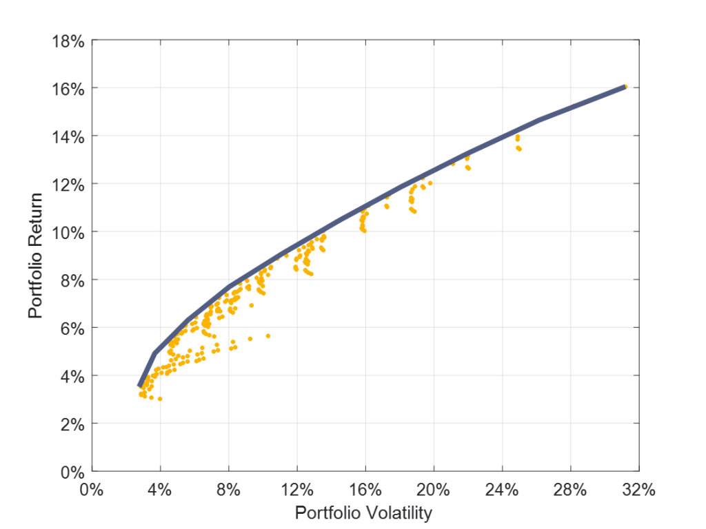
Own calculations from SBBI Yearbook data available from Morningstar and Ibbotson Associates. Data from 1926-2022. Indices are not available for direct investment. Past performance is no guarantee of future returns.
As a general statement, for a given level of risk, investors prefer a higher level of expected return. And for a given level of expected return, investors prefer a lower level of risk. This means that a “rational” investor (within the framework of MPT – and we’ll talk about this in a few minutes) will want to select one of the portfolio at the upper left edge. These are the portfolios where they will have the highest level of return at a given level of risk (or vice versa if they are focusing on achieving a specific level of expected return).
If we accept the assumptions made as part of the MPT, there is no reason to ever select a portfolio that is not on the efficient frontier. The big decision that is left to the investor will be to select their desired level of risk, and then invest according to the model outputs.
Problems with Modern Portfolio Theory
We now understand that there are serious issues with using MPT to determine investment portfolios for household investors, especially after retirement begins. Harry Markowitz recognized this. After winning the Nobel Prize in 1990, he was asked to write an article in 1991 for the first issue of Financial Services Review about how MPT applies to household investors. This article was named, “Individual versus Institutional Investing.” In the article, he writes about how he had never thought about the household’s investing problem before, and after reflecting on it for an evening, he realized that households face a very different investing problem from the large institutional investors, such as mutual funds, he had in mind when developing MPT. MPT does not teach how individual households should build investment strategies to meet their lifetime financial planning goals.
Namely, and this is really the key for understanding how the retirement income problem differs from the MPT approach, households must meet spending goals over an unknown length of time in retirement. MPT just seeks how to grow wealth over a single time period, such as a year, when there is no need to take distributions from the portfolio. It is an assets-only model. The preretirement wealth accumulation notion that households seek to grow wealth is more closely aligned with MPT, but the retirement income problem is vastly different. There may surely be a relationship between the idea that having more wealth will support more spending, and the idea that building diversified portfolios is still valid, but that relationship is more complicated when it is unknown how long the spending must last and when taking distributions from assets works to amplify the impacts of investment volatility on the retirement income plan.
With sequence risk for portfolio distributions, the extra shares sold to meet a spending goal when markets are down are no longer available to experience the growth of any subsequent market recovery. The point chosen on the efficient frontier can be different when viewed in the context of the household’s problem, and there can be a role for annuities or other risk management tools that are not included as asset classes in traditional MPT. Simply, MPT does not account for cash flows or longevity risk. It equates risk with short-term asset volatility rather than with the ability to meet financial goals.
Risk in the context of the household’s investing problem is only tangentially related to the volatility or standard deviation of returns. Volatility is important in that it relates to risk tolerance and whether individuals can handle the short-term volatility of their portfolio. If greater volatility leads them to not stick with their financial plan, then this must be incorporated into the asset allocation decision. But more generally, risk for the household relates to the ability to meet financial goals over a long-term planning horizon.
A low-volatility portfolio offering insufficient return potential can ensure failure for the financial plan. This is riskier from the household’s perspective than a more volatile portfolio that supports a higher probability of success for the financial plan. A key difference between probability-based and safety-first approaches is that the probability-based approach is more comfortable with accepting greater volatility for higher return potential and an improved chance for success, while the safety-first approach looks for alternatives that do not expose core retirement spending goals to market volatility. The question is ultimately about which is the best way to be able to spend more than a bond ladder can support: to rely on the excess returns expected to be provided by the stock market, or to rely on the power of risk pooling to bring additional spending power to those facing a higher cost retirement.
In addition to all of these issues, there is also the problem of predicting the inputs needed to generate the efficient frontier. While many investors use historical returns (as we did earlier on), there is a reason that financial services sales material is littered with disclaimers stating that “Past performance is not a guarantee of future returns.”
If we are not able to arrive at accurate risk, return, and cross correlation estimates for each asset class the then efficient frontier – and resulting asset allocations – will not represent the “optimal” portfolio. It is the classic “Garbage in, Garbage out” problem.
What Use is MPT?
The obvious question after walking through the limitations of Modern Portfolio Theory, is why is it worth discussing? If there are so many substantial problems with the theory, does it have any use?
Yes. Even acknowledging all of it’s issues, MPT is one of the most important ideas in finance and investing.
We may not be able to use MPT to design the “optimal” portfolio, but the fundamental insight – that portfolios need to be considered on a holistic basis – is absolutely crucial for both your investment portfolio, and your broader retirement income plan.
The two big takeaways – that you need to look at individual investments in the context of your broader portfolio, and that combining risky assets can make you overall portfolio less risky in total – are the driving forces in how we view portfolio construction to this day.