Diversification is a vital tool for mitigating the level of risk in your portfolio while investing, but it can also be used when considering your withdrawal rate and spending in retirement.
Safe withdrawal rates are connected in vitally important ways to underlying asset class choices and their return/volatility characteristics. Often, retirees are limited to accepting whatever a researcher assumes about market returns in order to obtain guidance about sustainable spending rates.
I talked about why I found this troubling in my article “Capital Market Expectations, Asset Allocation, and Safe Withdrawal Rates” from 2012. It provides a framework for connecting these pieces together, in turn letting retirees move beyond existing research assumptions to identify a more personalized safe withdrawal rate.
Reconciling the assumptions underpinning safe withdrawal rate studies with your own capital market expectations and constraints is a daunting task.
My article proposed a general framework for determining a safe withdrawal rate for a given retirement duration, acceptable failure probability, asset allocation, and capital market expectations. Retirees do not need to be constrained by the assumptions and choices of others.
Most researchers use one set of capital market expectations to study aspects of safe withdrawal rates. Often, they base their analyses on U.S. historical data going back to 1926. This is far from a perfect solution.
When determining a forward-looking safe withdrawal rate, the most important factor is our expectations about future market returns as driven by their underlying components: income, growth, and changes in valuation multiples
If current bond yields are noticeably lower than usual, the average historical bond return will likely be of little relevance.
But not all research is based on historical averages. Sometimes researchers use different assumptions, either because they want to illustrate a particular concept with basic assumptions, or because they have incorporated their own capital market expectations.
Still, a general problem remains: safe withdrawal rates research leaves unanswered questions about what would happen if different asset classes are included, or if different assumptions are made about returns, volatilities, and correlations.
My research generalized the framework for safe withdrawal rates, presenting a structure that incorporates user-specified capital market and retirement assumptions.
I used Monte Carlo simulations to calculate the combinations of real portfolio arithmetic returns and volatilities that would support different withdrawal rates for various retirement durations and acceptable failure probabilities.
From there, it is a matter of determining the portfolio’s expected return and volatility based on our assumptions about asset classes and their expected returns, volatilities, and correlations. In order to find the optimal asset allocation, these assumptions can be transformed into an efficient frontier.
Overlaying the efficient frontier onto my exhibits lets you find the point corresponding to the highest maximum sustainable withdrawal rate. The asset allocation for the optimal point can then be determined separate from the underlying efficient frontier characteristics.
This provides you with a recommended withdrawal rate and recommended asset allocation for your own specifications.
My article also described a secondary finding: that a wide range of asset allocations support withdrawal rates nearly as high as the optimal asset allocation.
Many retirees will be able to support a withdrawal rate within 0.1 percentage point of the optimum with a markedly lower stock allocation. Conservative retirees need not be pressured into uncomfortably aggressive asset allocations, such as the recommendations for 50 to 75 percent stocks found in prominent research articles by Bill Bengen and others.
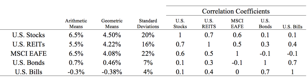
Exhibit 1 provides capital market assumptions for five asset classes: U.S. stocks, U.S. REITs, the MSCI EAFE for international stocks, U.S. bonds, and U.S. bills. These include the arithmetic real returns, compounded returns, volatilities, and correlations. These are not my recommended assumptions—they are a case study about the process.
Assuming that these values align with a retiree’s viewpoints and choices for asset allocation, Exhibit 1 provides the ingredients to study sustainable spending rates.
Exhibit 1
Hypothetical Long-term Capital Market Expectations
(in real U.S. Dollar terms)
Hypothetical Long-term Capital Market Expectations
Note: These are hypothetical numbers used to illustrate the framework for expanding the asset allocation that can be used with sustainable spending studies. They do not represent actual forecasts.
To assess the importance of these different capital market expectations, I compute an efficient frontier for this set of assumptions. Software is available to make such computations, as this task is generally not done by hand. Mean-variance optimizer software uses inputs to find the efficient frontier of asset allocations that provide the most return for a given volatility or the least volatility for a given return.
The efficient frontier can then be plotted onto the grid framework relating withdrawal rates to returns and volatilities for an acceptable failure probability and retirement duration.
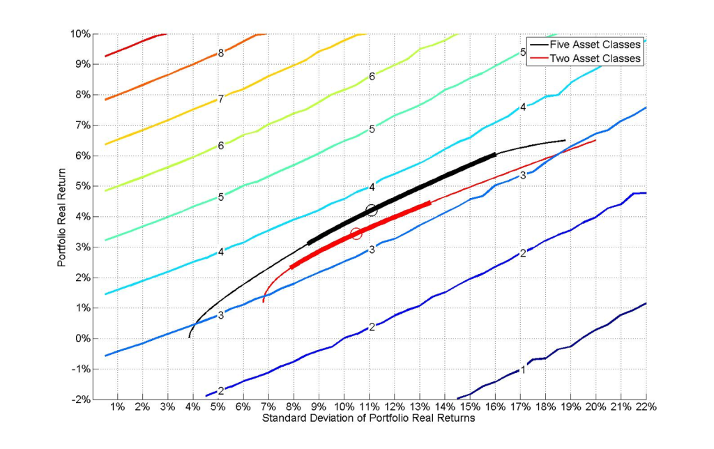
In Exhibit 2, I overlaid the efficient frontier (a lighter color for only considering U.S. stocks and bonds, black for all five asset classes in Exhibit 1) onto the withdrawal rate charts for a thirty-year retirement duration and a 10 percent acceptable failure probability (different charts can be made for different assumptions about retirement length and the acceptable failure rate).
Each diagonal line (technically an “isoquant”) shows the combination of rates-of-return and standard deviations that will support a given sustainable withdrawal rate.
From this overlay, we determine where the efficient frontier reaches to the highest withdrawal rate. The thin parts of the curves identify the entire efficient frontier of asset allocations.
The circles identify the points reaching to the highest sustainable withdrawal rate. The thick parts of the curves identify the range of portfolio allocations supporting withdrawal rates within 0.1 percentage points of the maximum.
Returning to the mean-variance optimization results, we find the asset allocation corresponding to this optimal point. The optimal asset allocation can then be compared to the retiree’s investment constraints and risk tolerance to determine its acceptability.
If it is found to be unacceptable, other points on the efficient frontier that support progressively lower withdrawal rates can be investigated until a suitable asset allocation is found.
Exhibit 2
Sustainable Withdrawal Rates with 10% Failure for 30-Year Retirement Horizon
Sustainable Withdrawal Rates with 10% Failure for 30-Year Retirement Horizon
Exhibit 3 provides further detail. When using all five asset classes (the black efficient frontier), the optimal asset allocation supports a 3.61 percent withdrawal rate over thirty years with a 10 percent chance for failure. The optimal asset allocation is shown.
Meanwhile, when only two of the asset classes are used, the withdrawal rate is 3.34 percent with an optimal asset allocation of 47.2 percent stocks and 52.8 percent bonds. The asset allocations provided in Exhibit 3 cannot be seen in the visual found in Exhibit 2, but they exist behind the scenes within the software.
Sustainable Withdrawal Rates with 10% Failure for 30-Year Retirement Horizon
| Asset Classes | Withdrawal Rate | Real Portfolio Return | Portfolio Standard Deviation | Asset Allocation |
| U.S. Stocks | 3.34% | 3.4% | 10.5% | 47.2% |
| U.S. Bonds | 52.8% | |||
| With Five Asset Classes | ||||
| Asset Classes | Withdrawal Rate | Real Portfolio Return | Portfolio Standard Deviation | Asset Allocation |
| U.S. Stocks | 3.61% | 4.2% | 11.1% | 14.9% |
| U.S. REITS | 30.5% | |||
| MSCI EAFE | 20.4% | |||
| U.S. Bonds | 34.2% | |||
| U.S. Bills | 0.0% | |||
Withdrawal Rates with 10% Failure for 30-Year Retirement Horizon
This case study illustrates how the framework for incorporating your own capital market expectations works. Of course, formulating appropriate capital market expectations is hard. Volatility especially complicates the process.
A common view is that future stock returns will be lower than historical averages, but what about stock volatility? Would lower stock returns be accompanied by lower volatility, or is it reasonable to keep volatility the same? Might we even expect volatility to increase?
The withdrawal rate lines in Exhibit 2 are upward sloping, making pinpointing the precise combination of expected returns and volatilities especially important; if you forecast lower volatility, you can spend more for a given level of returns.
This framework can be used to estimate sustainable withdrawal rates for a given failure rate and retirement duration for most any kind of capital market expectations.
The purpose here is to demonstrate how retirees can translate their own expectations into an understanding about how to choose a withdrawal rate and asset allocation strategy.